-
Flow-based generative model(NICE, Real NVP, Glow 논문리뷰)논문 리뷰/Generative Model 2024. 6. 21. 14:12
flow-based generative의 시작에 있어 매우 중요한 세 개의 논문 NICE, Real NVP, Glow에 대해 리뷰해보고자 한다.
그 전에, 먼저 flow-based generative model 관련 기초 개념에 대해서 설명하고자 한다.
※ 기초 개념은 출처 [1] https://lilianweng.github.io/posts/2018-10-13-flow-models/
Flow-based Generative Model
Flow-based generative model은 GAN, VAE 같은 다른 generative model과 다르게 invertible한 transformations를 쌓아서 만든다. 또한 data distribution $p(x)$를 학습하며, loss function은 negative log-likelihood로 심플하다.
$p(x)$를 explicit하게 안다는 것은 이 모델의 큰 특징이자 장점이며, GAN의 경우 분포를 통해 학습하지 않으며 VAE는 log-likelihood를 최대화하지 못하고 lower bound인 ELBO(the evidence lower bound)를 학습한다.
선형대수 복습
Jacobian matrix and Determinant
Jacobian matrix $J$는 $f : R^n \rightarrow R^m$으로 가는 함수에 대해 일차 미분을 matrix 형태로 써놓은 것으로 각각의 원소 $J_{ij} = \frac{\partial f_i}{\partial x_j}$이다.
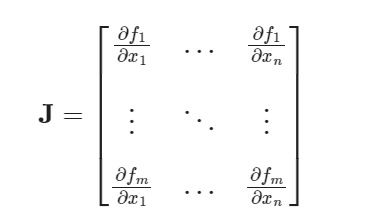
Jacobian matrix 여기서 J가 정사각행렬일 때, 즉 $m=n$일 때 J의 행렬식을 Jacobian determinant라고 부른다. Jacobian determinant는 함수 $f$의 중요한 성질을 나타낸다.
(1) (inverse function theorem)The function $f$ has a differentiable inverse function in an neighborhood of a point $x$ iff the Jacobian determinant is nonzero at $x$
(2) The absolute value of Jacobian determinant gives us the factor by which the function $f$ expands or shrinks volumes near $x$.
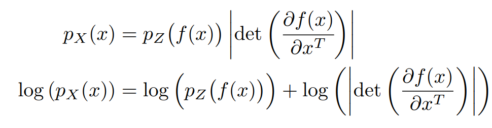
Change of Variable Theorem
확률 변수 $z$의 확률밀도함수를 $\pi(z)$라 두자. 역함수가 존재하는 함수 $f$에 대해 $x = f(z)$라 정의하면 확률 변수 $x$의 확률밀도함수 $p(z)$는 다음과 같이 나타낼 수 있다.
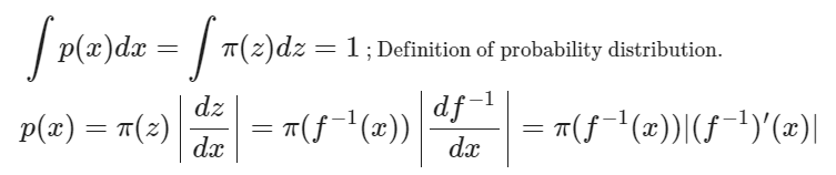
one dimension 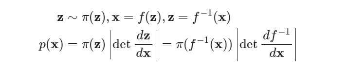
multi dimension Normalizing Flows
Normalizing flow는 간단한 분포를 invertible한 transformation을 여러번 태워 복잡한 분포로 만들 수 있다는 아이디어에 기반한다.
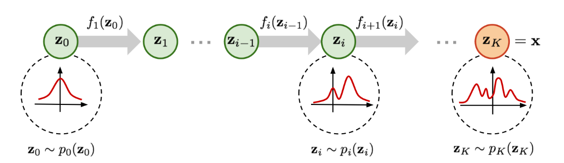
이 과정에서 chage of variable을 통해 확률변수 $x$의 분포를 $z$의 분포로 쓸 수 있다. (과정 생략)
$\log p(x) = \log \pi_{0} (z_0) - \sum_{i = 1}^{K} \log |det \frac{df_i}{dz_{i-1}}|$
여기서 $z_{i-1}$이 $z_i$로 가는 과정을 flow라고 부르며 $\pi_i$로 나타내는 연속적인 chain을 normalizing flow라고 부른다.
Models with Normalizing Flows
Exact log-likelihood of $\log p(x)$를 알 수 있기 때문에 우리는 negative log-likelihood(NLL)를 maximize하는 방향으로 학습하면 된다. (tractable하다는 특징 덕분에 GAN이나 VAE보다 학습하기 쉽다고 한다.)

['15 ICLR] NICE : Non-Linear Independent Components Estimation
A good representation is one in which the distribution of the data is easy to model
데이터 $x$에서 $h$로 가는 함수 $f$를 생각해보자. 즉, $h = f(x)$이다.

chage of variable 여기서 함수 $f$는 두가지 조건을 만족해야 한다.
1. Jacobian determinant를 쉽게 계산할 수 있을 것
2. 함수 $f$의 역함수를 쉽게 구할 수 있을 것
Goal : 확률분포 ${p_{\theta}, \theta \in \Theta}$에서 $\theta$ 학습하기
$p_X(x)$는 다음과 같이 쓸 수 있기 때문에 likelihood를 최대화하므로써 학습할 수 있다.
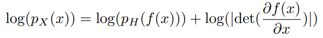
$p_X(x)$은 posterior distribution으로 우리가 알고자 하는 분포이며, $p_H(x)$는 prior distribution으로 우리가 정의하는 분포이다. prior distribution은 factorize될 수 있는 분포를 고르며, 이 논문에서는 isotropic Gaussian distribution을 골랐다.
* isotropic Gaussian distribution은 covariance matrix가 $\sigma^2 I$인 분포로 각각의 차원이 독립이지만 분산은 동일한 분포이다.
그러면 우리는 아래와 같이 non-linear independent components estimation(NICE) criterion을 얻을 수 있다.

위 식에서 함수 $f$의 Jacobian determinant의 값이 커지길 원하기 때문에 Jacobian determinant는 수축에 패널티를 주고, 확장을 유도하는 역할을 한다.
Architecture
General coupling layer

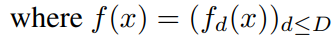
$x = (x_{I_1}, x_{I_2})$로 나누고, $x_{I_1}$의 차원은 $|I_1|$, $x_{I_2}$의 차원은 $|I_2|$라 하자. $x \rightarrow y$로 가는 매핑을 위와 같이 정의할 수 있다. 여기서 우리는 $g$를 아래와 같이 정의하며, coupling law라고 부른다.

Jacobian matrix와 determinant는 아래와 같이 표현 가능하다.

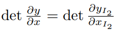
역변환 역시 간단하게 아래와 같이 나타낼 수 있으며, 우리는 위와 같은 변환을 a coupling layer with coupling function m이라고 부른다.
Additive coupling layer
:General coupling layer에서 additive function $g(a;b) = a+b$
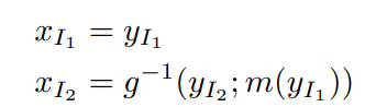
$a = x_{I_1}$, $b = m(x_{I_1})$이라고 정의하자.
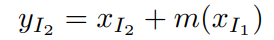
이 경우 $g^{-1}$가 아래와 같이 나타나기 때문에 inverse of $g$가 굉장히 심플하게 표현된다.

또한 여기서 coupling function $m$은 어떤 함수를 고르든 Jacobian matrix에 영향을 주지 않으므로 $m : R^d \rightarrow R^{D-d}$은 복잡한 neural network를 골라 학습할 수 있어 모델의 유연성이 올라간다.
Additive coupling layer는 unit Jacobian determinant를 가지고 있다. 이 논문에서는 Additive coupling layer를 골라 실험을 진행하였다.
* 다른 coupling law로는 affine coupling law $g(a; b) = a * b_1 + b_2$가 있다. 여기서 $a * b$는 multiplicative coupling law를 가르킨다.
Combining coupling layers
여러개의 coupling layer를 쌓아 복잡한 layered transformation을 만들었으며, coupling layer는 입력 파트의 일부 위치를 바꾸지 않으므로($y_{I_1} = x_{I_1}$인 파트) 모든 차원이 뒤섞여 학습이 되기 위해서는 두 개의 파트로 나누어진 입력이 위치가 바뀔 수 있도록 해야한다. 이 논문에서는 모든 차원이 서로 영향을 주기 위해 최소 3개의 coupling layer가 필요하다고 설명한다.
Allowing Rescaling
Additive coupling layer의 단점은 unit Jacobian detereminant를 갖는다는 것이다. 이는 volume preserving한다는 의미로 압축과 확장을 통해 데이터의 feature를 잡아내는 딥러닝의 특성과 맞지 않는다고 할 수 있다. 이러한 단점을 극복하기 위해 a diagonal scaling matrix S를 가장 윗 레이어에 추가했다. diagonal 파트만 있기 때문에 아래와 같이 변환시킨다.
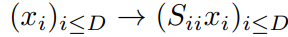
$i$에 따라 $S_{ii}$의 값이 다르기 때문에, $S_{ii}$ 값에 따라 각 차원에 부여하는 가중치가 달라진다.
$S_{ii}$가 커지는 경우 i번재 차원은 덜 중요하다고 학습이 되었으며, $log(|S_{ii}|)$때문에 $S_{ii}$가 0으로 가는 것을 막아준다.
실험 결과
['17 ICLR] Density Estimation Using Real NVP
NICE에서 사용한 Change of Variable을 똑같이 사용한다. notation이 살짝 바뀌었는데, NICE에서는 hidden layer을 H로 표현했다면 Real NVP에서는 Z로 표현하였다.
Affine coupling layer
NICE에서 additive coupling layer를 선택했다면, Real NVP에서는 Affine coupling layer를 선택하였다.

여기서 $s$와 $t$는 scale과 translation을 의미하며 $R^d \rightarrow R^{D-d}$인 함수이다.
이 함수는 invertible하며 inverse 또한 쉽게 구할 수 있다.

여기서 inverse를 쉽게 구할 수 있다는 말은 sampling이 inference만큼 쉽게 구해진다는 것으로 이해할 수 있다.
Jacobian matrix and determinant
Affine coupling layer로 표현된 transform의 Jacobian matrix와 determinant는 다음과 같다.

Jacobian matrix 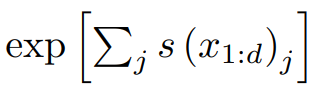
Jacobian determinant Jacobian determinant에 $s$나 $t$에 대한 복잡한 연산이 포함되지 않았기 떄문에 우리는 $s$와 $t$ 함수를 고르는데 제약이 없다. 그래서 논문에서는 $s$와 $t$를 복잡한 neural network로 골라 학습시켰다.
masked convolution
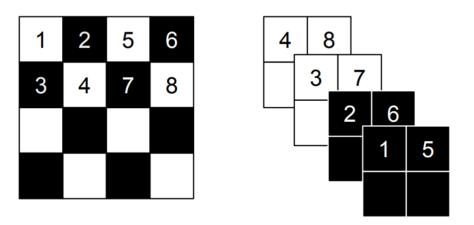
왼쪽은 spatial checkboard pattern mask, 오른쪽은 channel-wise pattern mask 
b를 mask라고 했을 때 다음과 같이 마스크를 사용한다.
더보기질문 : mask를 어떻게 사용했다는걸까?
Multi-scale architecture

The squeezing operation transforms coupling layers with alternating checker boards * 3
→ squeezing operation
→ coupling layers with alternating channel-wise maskings* 3
→ coupling layers with alternating checker boards * 3
 더보기
더보기질문 : checker board mask는 size를 줄이는걸까?
inference의 의미
Batch normalization
running average over recent minibatches에 대해 batch normalization을 진행했다. 또한 batch normalization을 모든 coupling layer output에 적용하므로서 Jacobain computation을 용이하게 했다.
rescaling function rescaling function의 Jacobian determinant는 다음과 같다.

Jacobian determinant 실험 결과
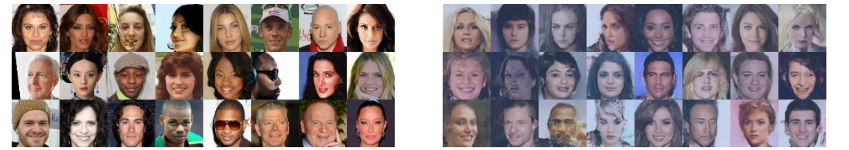
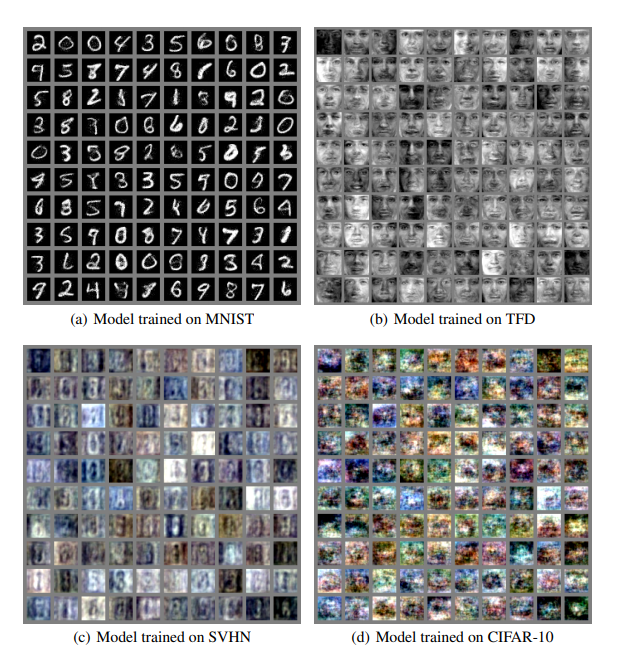
왼쪽 : 데이터 셋, 오른쪽 : 학습된 모델로부터 뽑은 샘플들 ['18 NeurIPS] Glow : Generative flow with invertible 1x1 convolutions
Glow는 RealNVP에 더하여 $1 \times 1$ convolution을 사용해 성능을 향상시킨 모델이다. 사람의 얼굴을 상당히 사실적으로 생성할 수 있게 한 모델로, GAN과 VAEs에 비해 관심을 받지 못한 flow-based generative model을 떡상시킨 논문이라고도 할 수 있다.
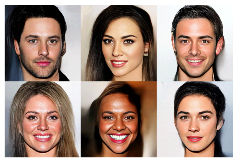
머리카락 부분은 엉성하지만, 얼굴이 매우 사실적으로 생성되었다. 더보기$x$가 연속인 경우, 우리는 목적함수를 negative log-likelihood를 아래와 같이 쓸 수 있다고 한다.(왜?)
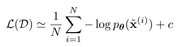

where $a$ is determined by the discretization level of the data,
$M$ is the dimensionality of $x$
Architecture
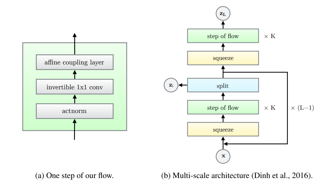
Actnorm
Real NVP에서는 batch normalization 방법을 사용해 정규화를 진행했다. 하지만 batch normalization에 의해 추가되는 노이즈 분산은 GPU당 미니배치 또는 PU(processing unit)의 크기와 반비례하기 때문에 PU당 작은 미니배치의 크기는 성능을 저하시킨다고 알려져있다. 하지만 우리는 큰 이미지를 다루므로 배치를 작게 설정할 수 밖에 없다.
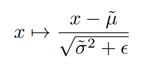
그래서 우리는 actnorm layer(for activation normalization)을 제안했다. actnorm에서는 각 채널에 대해 scale과 bias parameter를 설정하고 일종의 affine transform처럼 작동한다.
여기서 초기화 방법이 중요한데, 처음에는 initial minibatch of data에 대한 actnorm의 출력의 채널당 평균과 분산이 각각 0과 1이 되도록 설정한다. 그 다음에는 scale과 bias가 data와 독립인 변수로 취급하고 학습 가능한 변수로 생각한다. 이러한 초기화 방법은 data dependent initialization이라는 방법론으로 Salimans와 Kingma가 2016년 제안한 방법이다.
Invertible $1 \times 1$ convolution
input $x$를 두 개의 부분으로 나눠 $x_{1:d}$부분은 항등변환하기 때문에 제대로 학습되지 않을 가능성이 있다. Real NVP 에서는 mask, 즉 고정된 permutation을 통해 각 차원을 섞어주었다면, 이 논문에서는 invertible $1 \times 1$ convolution을 사용한다. 이 convolution은 permutation의 generalization으로 생각할 수 있다.
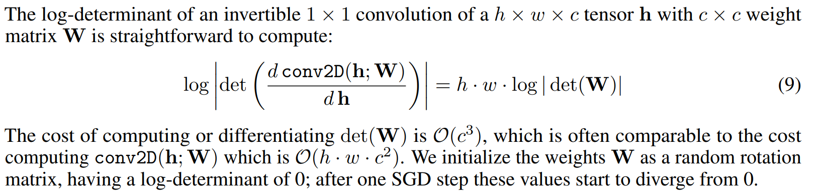 더보기
더보기질문 : 왜 W는 c*c matrix이지?
$det(W)$는 계산복잡도가 일반적으로 $O(c^3)$으로 알려져있다. 이러한 복잡한 계산을 단순화하기 위해 LU decomposion을 사용했다.
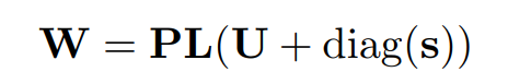
P는 permutation matrix, L은 대각선이 1인 lower triangle matirx, U는 대각선이 0인 upper triangle matrix

이렇게 계산하면 $O(c)$로 $det(W)$를 계산할 수 있다.
실험 결과

Reference
[1] https://lilianweng.github.io/posts/2018-10-13-flow-models/
: 굉장히 잘 쓰여진 블로그로 한번 읽어보길 강추!! Jacobian matrix나 행렬 자체가 어려운 분들이 읽기 쉽게 설명해두었다.
[2] https://en.wikipedia.org/wiki/Jacobian_matrix_and_determinant
[3] https://arxiv.org/abs/1410.8516
NICE: Non-linear Independent Components Estimation
We propose a deep learning framework for modeling complex high-dimensional densities called Non-linear Independent Component Estimation (NICE). It is based on the idea that a good representation is one in which the data has a distribution that is easy to m
arxiv.org
[4] https://arxiv.org/pdf/1605.08803
[6] 1x1 convolution https://hwiyong.tistory.com/45
1x1 convolution이란,
GoogLeNet 즉, 구글에서 발표한 Inception 계통의 Network에서는 1x1 Convolution을 통해 유의미하게 연산량을 줄였습니다. 그리고 이후 Xception, Squeeze, Mobile 등 다양한 모델에서도 연산량 감소를 위해 이 방
hwiyong.tistory.com
'논문 리뷰 > Generative Model' 카테고리의 다른 글