-
Sliced Score Matching 논문 리뷰(Sliced Score Matching : A Scalable Approach to Density and Score Estimation)논문 리뷰/Generative Model 2024. 7. 31. 18:00
Score-based model을 공부하다가 denoising score matching과 더불어 sliced score matching이 나와 논문 리뷰를 해보고자 한다. 이 논문은 수학 증명이 탄탄하게 받혀주는 논문인데, 간단하게 statement 위주로 정리해보고자 한다.
※ 읽기에 앞서 score function 관련 내용에 대한 사전 지식이 필요하다. 관련 내용은 Score-based models 포스팅을 통해 확인할 수 있다.
Introduction
Score matching (Hyvärinen, 2005) is particularly suitable for learning unnormalized statistical models, such as energy based ones. It is based on minimizing the distance between the derivatives of the log-density functions (a.k.a., scores) of the data and model distributions.Unlike maximum likelihood estimation (MLE), the objective of score matching only depends on the scores, which are oblivious to the (usually) intractable partition functions. However, score matching requires the computation of the diagonal elements of the Hessian of the model’s log-density function. This Hessian trace computation is generally expensive (Martens et al., 2012), requiring a number of forward and backward propagations proportional to the data dimension. This severely limits its applicability to complex models parameterized by deep neural networks, such as deep energy-based models (LeCun et al., 2006; Wenliang et al., 2019).
Introduction에 완벽하게 score matching에 대해 설명이 있어 원문 그대로 가져왔다. (관련 내용은 score-based model 포스팅에서 확인 가능합니다.)
Sliced score matching 기법에서 중요한 직관은 고차원의 score를 바로 추정하는 것이 아니라, score의 random한 방향으로의 projection을 고려한다는 점이다.
Background

notation과 setting은 다음과 같다.
이론적으로 Z(θ)는 잘 정의되어 있지만, 실제로 Z(θ)를 계산하는 것은 거의 불가능에 가깝다.
따라서 pm 식 양 변에 log를 씌워 score를 정의하게 되면 score function은 partition function Zθ와 독립이 되므로, 논의가 훨씬 용이해진다.
score matching에서는 Fisher divergence를 이용해 objective를 아래와 같이 나타낸다.
여기서 score function of the data sd(x)는 알 수 없으므로, 위 식은 다음과 같이 바꿀 수 있다.
(L(θ)=J(θ)+constant)
J(θ)는 unbiased estimator로 ~pm를 학습하는데 사용할 수 있다.
위 식은 log-density function의 Hessian의 trace term을 포함하고 있으며, Hessian의 trace를 계산하기 위해서는 D(=input의 차원)번의 backpropagation을 sm에 적용하여 각각의 대각선 term을 구해야 한다. 일반적으로 D는 10^6 정도의 값을 가지기 때문에 이는 학습을 상당히 느리게 만든다.
☞ 이것이 바로 Sliced Score Matching 기법이 나오게 된 배경이다!
implicit distribution은 sampling process는 가능하지만, tractable한 density를 알기는 어려운 density를 의미한다. GAN이 대표적으로 implicit distribution에 의해 작동하는데, sliced score matching은 implicit distribution의 score를 구하는데도 용이하다.
아래와 같은 상황을 생각해보자. 다음과 같은 식의 변형을 통해 우리는 H(q(θ(x))의 gradient w.r.t. θ를 다음과 같이 구할 수 있으며, score은 intractable하지만 이를 score estimation을 통해 구할 수 있다.
Sliced Score matching
이 논문은 저차원의 문제가 고차원의 문제보다 다루기 쉽다는 점에서 착안해서 score function의 projection을 score function 대신 objective function에 대입해보았다. 앞에서 제안된 L(θ)를 다시 쓰면 아래와 같은데,
여기서 random vector v는 pv를, x는 pd를 따르며 독립이고, Epv[vvT]>0, Epv[||v||22]<inf이다. 위 조건을 만족하는 pv의 선택폭은 상당히 넓은데, 잘 알려진 분포로는 multivariate standard normal(N(0,ID), multivariate Rademacher distribution 또는 uniform distribution on the hypersphere 등을 고를 수 있다.
L(θ;pv) 식을 integration by parts로 J(θ;pv)로 바꾸면 아래와 같이 정의할 수 있다.

그리고 Theorem 1에 의해 L(θ;pv)=J(θ;pv)+C임을 다시금 증명할 수 있다.

학습 시 우리는 N개의 샘플에 대해 M개의 vector v에 대한 projection을 상정하므로 아래와 같이 unbiased estimator of ˆJ를 생각할 수 있다.

만약 우리가 pv를 multivariate standard normal 또는 multivariate Rademacher distribution을 고른다면 vector v의 L2 norm은 1이므로 아래와 같이 식을 간소화하여 variance를 줄일 수 있다.

이 논문에서는 실험적으로 $\hat{J_{vr} 이\hat{J}$에 비해 좋은 성능을 보여줬다고 주장한다.(이하 SSM-VR로 부르자)
Slice score matching을 도입하므로서 더이상 Hessian의 trace를 계산해야 하는 번거로움을 덜 수 있다. Sliced score matching 역시 Jacobian-vector product term을 포함하기 때문에 시간이 오래 걸리지는 않을까 생각할 수 있는데, 아래 알고리즘을 이용하면 M+1번의 연산으로 gradient를 구할 수 있다. (M는 vector v의 갯수) M의 크기와 variance는 trade off 관계인데, 이 논문에서는 M= 1일 때를 상정하고 실험했다.

score estimation을 위해 deep neural network h(x;θ)를 ˆJ에 대입해서 생각해보자.

위 식을 최적화하는 θ를 찾으면 h(x;ˆθ)는 data distribution의 score를 근사한다.

Theoretical Analysis
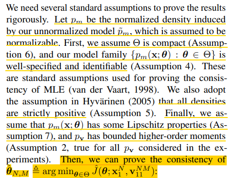
Sliced score matching기법이 얼마나 안정적인지를 보여주는 증명들이다. 증명은 생략하였고, 더보기 란에 필요한 assumption들을 달아놓았다.
 더보기
더보기이 증명을 위해서는 아래의 가정들이 필요하다.
 더보기
더보기이 증명을 위해서는 아래의 추가 가정이 필요하다.

Related work
이 논문에서는 Hessian의 trace term을 계산하기 않기 위해 발전한 다양한 방법들을 소개하고 있다. 이 중 Denoising Score Matching은 유명해서 한 번쯤 읽어보면 좋을 것 같다. 관련 포스팅을 정리해놓은 것으로 Denoising Score Matching에 대한 설명은 갈음하고자 한다.
- Denoising Score Matching
- Approximate Backpropagation
- Curvature Propagation
실험은 타 score matching 기법과 비교 실험 및 다양한 활용 방법을 소개하고 그 성능을 입증하였으나 오늘의 논문 리뷰에서는 생략한다.
'논문 리뷰 > Generative Model' 카테고리의 다른 글
