-
[3] pykan 라이브러리 사용법 : Examples카테고리 없음 2024. 10. 14. 22:24Kolmogorov-Arnold Network(KAN)을 가장 쉽게 사용할 수 있는 방법! pykan 라이브러리 사용법에 대해 정리해보고자 한다.
※ 모든 내용은 https://kindxiaoming.github.io/pykan/intro.html 의 내용을 번역한 것으로 모든 저작권은 해당 페이지에 있습니다. 부정확한 표현이 있을 수 있으니 원문 페이지를 꼭 참고해주세요!
Example 1 : Function Fitting
이번 예제에서는 그리드를 세분화하여 KAN의 함수 적합 능력을 극대화해보고자 한다.
from kan import *


device = torch.device('cuda' if torch.cuda.is_available() else 'cpu')
print(device)

# initialize KAN with G=3
model = KAN(width=[2,1,1], grid=3, k=3, seed=1, device=device)

# create dataset
f = lambda x: torch.exp(torch.sin(torch.pi*x[:,[0]]) + x[:,[1]]**2)
dataset = create_dataset(f, n_var=2, device=device)

model.fit(dataset, opt="LBFGS", steps=20);
>> | train_loss: 1.42e-02 | test_loss: 1.43e-02 | reg: 1.16e+01 |
여기서 좀 더 세밀한 KAN으로 설정해보자.
# initialize a more fine-grained KAN with G=10
model = model.refine(10)
model.fit(dataset, opt="LBFGS", steps=20);
>> | train_loss: 9.52e-04 | test_loss: 9.80e-04 | reg: 1.16e+01 |
loss가 더 좋아진 것을 확인할 수 있다. grid를 더 finer하게 수정해보자.
더보기refine(new_grid) : grid refinement
Args:
new_grid : initthe number of grid intervals after refinement
Returns:
a refined model : MultKAN
Example
>>> from kan import *
>>> device = torch.device('cuda' if torch.cuda.is_available() else 'cpu')
>>> model = KAN(width=[2,5,1], grid=5, k=3, seed=0)
>>> print(model.grid)
>>> x = torch.rand(100,2)
>>> model.get_act(x)
>>> model = model.refine(10)
>>> print(model.grid)
checkpoint directory created: ./model
saving model version 0.0
5
saving model version 0.1
10
grids = np.array([3,10,20,50,100]) train_losses = [] test_losses = [] steps = 200 k = 3 for i in range(grids.shape[0]): if i == 0: model = KAN(width=[2,1,1], grid=grids[i], k=k, seed=1, device=device) if i != 0: model = model.refine(grids[i]) results = model.fit(dataset, opt="LBFGS", steps=steps) train_losses += results['train_loss'] test_losses += results['test_loss']plt.plot(train_losses) plt.plot(test_losses) plt.legend(['train', 'test']) plt.ylabel('RMSE') plt.xlabel('step') plt.yscale('log')
n_params = 3 * grids
train_vs_G = train_losses[(steps-1)::steps]
test_vs_G = test_losses[(steps-1)::steps]
plt.plot(n_params, train_vs_G, marker="o")
plt.plot(n_params, test_vs_G, marker="o")
plt.plot(n_params, 100*n_params**(-4.), ls="--", color="black")
plt.xscale('log')
plt.yscale('log')
plt.legend(['train', 'test', r'$N^{-4}$'])
plt.xlabel('number of params')
plt.ylabel('RMSE')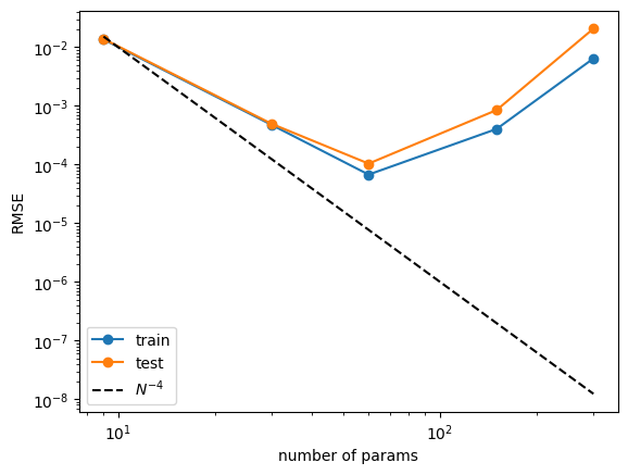
Example 3 : Deep Formulas
Tree-layer KAN
from kan import *

device = torch.device('cuda' if torch.cuda.is_available() else 'cpu')
print(device)

# create a KAN: 2D inputs, 1D output, and 5 hidden neurons. cubic spline (k=3), 5 grid intervals (grid=5).
model = KAN(width=[4,2,1,1], grid=3, k=3, seed=1, device=device)
f = lambda x: torch.exp((torch.sin(torch.pi*(x[:,[0]]**2+x[:,[1]]**2))+torch.sin(torch.pi*(x[:,[2]]**2+x[:,[3]]**2)))/2)
dataset = create_dataset(f, n_var=4, train_num=3000, device=device)

# train the model
model.fit(dataset, opt="LBFGS", steps=20, lamb=0.002, lamb_entropy=2.);

model = model.prune(edge_th = 1e-2)
model.plot()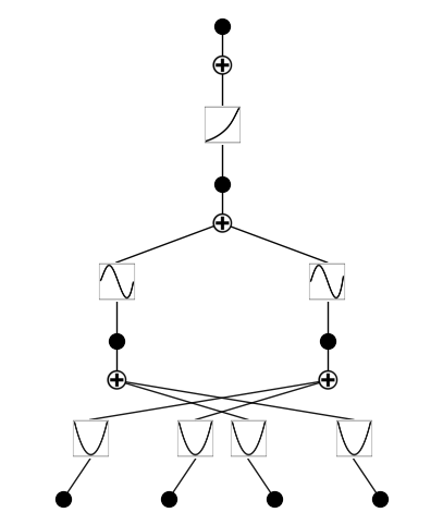
grids = [3,5,10,20,50]
#grids = [5]

train_rmse = []
test_rmse = []

for i in range(len(grids)):
    #model = KAN(width=[4,2,1,1], grid=grids[i], k=3, seed=0, device=device).initialize_from_another_model(model, dataset['train_input'])
    model = model.refine(grids[i])
    results = model.fit(dataset, opt="LBFGS", steps=50, stop_grid_update_step=20);
    train_rmse.append(results['train_loss'][-1].item())
    test_rmse.append(results['test_loss'][-1].item())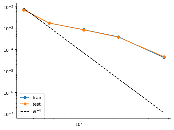
Two-layer KAN
이 예제에서는 2개의 KAN layer를 쌓는 것이 3개의 KAN layer를 쌓는 것보다 더 성능이 좋지 않다는 것을 보일 것이다.
from kan import KAN, create_dataset
import torch

# create a KAN: 2D inputs, 1D output, and 5 hidden neurons. cubic spline (k=3), 5 grid intervals (grid=5).
model = KAN(width=[4,9,1], grid=3, k=3, seed=0)
f = lambda x: torch.exp((torch.sin(torch.pi*(x[:,[0]]**2+x[:,[1]]**2))+torch.sin(torch.pi*(x[:,[2]]**2+x[:,[3]]**2)))/2)
dataset = create_dataset(f, n_var=4, train_num=3000)

# train the model
model.fit(dataset, opt="LBFGS", steps=20, lamb=0.002, lamb_entropy=2.);
model.plot(beta=10)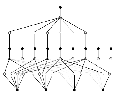
grids = [3,5,10,20,50]

train_rmse = []
test_rmse = []

for i in range(len(grids)):
    #model = KAN(width=[4,9,1], grid=grids[i], k=3, seed=0).initialize_from_another_model(model, dataset['train_input'])
    model = model.refine(grids[i])
    results = model.fit(dataset, opt="LBFGS", steps=50, stop_grid_update_step=30);
    train_rmse.append(results['train_loss'][-1].item())
    test_rmse.append(results['test_loss'][-1].item())
import numpy as np import matplotlib.pyplot as plt n_params = np.array(grids) * (4*9+9*1) plt.plot(n_params, train_rmse, marker="o") plt.plot(n_params, test_rmse, marker="o") plt.plot(n_params, 300*n_params**(-2.), color="black", ls="--") plt.legend(['train', 'test', r'$N^{-4}$'], loc="lower left") plt.xscale('log') plt.yscale('log') print(train_rmse) print(test_rmse)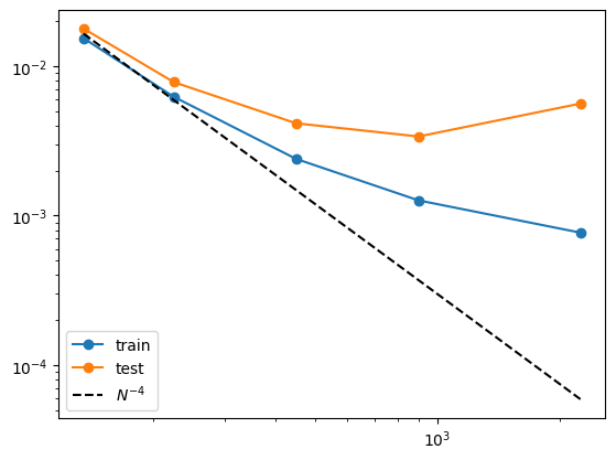
Example 4 : Classification
Regression formulation
regression problem(output dimension = 1, MSE loss) - 2개의 달 데이터 셋을 생성하자.
from kan import *
import matplotlib.pyplot as plt
from sklearn.datasets import make_moons
import numpy as np

device = torch.device('cuda' if torch.cuda.is_available() else 'cpu')
print(device)

dataset = {}
train_input, train_label = make_moons(n_samples=1000, shuffle=True, noise=0.1, random_state=None)
test_input, test_label = make_moons(n_samples=1000, shuffle=True, noise=0.1, random_state=None)

dtype = torch.get_default_dtype()
dataset['train_input'] = torch.from_numpy(train_input).type(dtype).to(device)
dataset['test_input'] = torch.from_numpy(test_input).type(dtype).to(device)
dataset['train_label'] = torch.from_numpy(train_label[:,None]).type(dtype).to(device)
dataset['test_label'] = torch.from_numpy(test_label[:,None]).type(dtype).to(device)

X = dataset['train_input']
y = dataset['train_label']
plt.scatter(X[:,0].cpu().detach().numpy(), X[:,1].cpu().detach().numpy(), c=y[:,0].cpu().detach().numpy())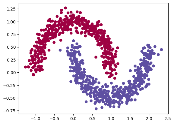
model = KAN(width=[2,1], grid=3, k=3, device=device)

def train_acc():
    return torch.mean((torch.round(model(dataset['train_input'])[:,0]) == dataset['train_label'][:,0]).type(dtype))

def test_acc():
    return torch.mean((torch.round(model(dataset['test_input'])[:,0]) == dataset['test_label'][:,0]).type(dtype))

results = model.fit(dataset, opt="LBFGS", steps=20, metrics=(train_acc, test_acc));
results['train_acc'][-1], results['test_acc'][-1]
>> (1.0, 0.9990000128746033)
lib = ['x','x^2','x^3','x^4','exp','log','sqrt','tanh','sin','tan','abs'] model.auto_symbolic(lib=lib) formula = model.symbolic_formula()[0][0] ex_round(formula, 4)>>
# how accurate is this formula?
def acc(formula, X, y):
    batch = X.shape[0]
    correct = 0
    for i in range(batch):
        correct += np.round(np.array(formula.subs('x_1', X[i,0]).subs('x_2', X[i,1])).astype(np.float64)) == y[i,0]
    return correct/batch

print('train acc of the formula:', acc(formula, dataset['train_input'], dataset['train_label']))
print('test acc of the formula:', acc(formula, dataset['test_input'], dataset['test_label']))
>>
train acc of the formula: tensor(1.)
test acc of the formula: tensor(1.)
Classification formulation
classification problem(output dimension = 2, CrossEntropy loss) - 2개의 달 데이터 셋을 생성하자.
from kan import KAN
import matplotlib.pyplot as plt
from sklearn.datasets import make_moons
import torch
import numpy as np

dataset = {}
train_input, train_label = make_moons(n_samples=1000, shuffle=True, noise=0.1, random_state=None)
test_input, test_label = make_moons(n_samples=1000, shuffle=True, noise=0.1, random_state=None)

dataset['train_input'] = torch.from_numpy(train_input).type(dtype).to(device)
dataset['test_input'] = torch.from_numpy(test_input).type(dtype).to(device)
dataset['train_label'] = torch.from_numpy(train_label).type(torch.long).to(device)
dataset['test_label'] = torch.from_numpy(test_label).type(torch.long).to(device)

X = dataset['train_input']
y = dataset['train_label']
plt.scatter(X[:,0].cpu().detach().numpy(), X[:,1].cpu().detach().numpy(), c=y[:].cpu().detach().numpy())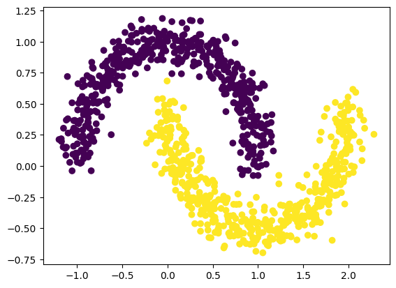
model = KAN(width=[2,2], grid=3, k=3, seed=2024, device=device)

def train_acc():
    return torch.mean((torch.argmax(model(dataset['train_input']), dim=1) == dataset['train_label']).type(dtype))

def test_acc():
    return torch.mean((torch.argmax(model(dataset['test_input']), dim=1) == dataset['test_label']).type(dtype))

results = model.fit(dataset, opt="LBFGS", steps=20, metrics=(train_acc, test_acc), loss_fn=torch.nn.CrossEntropyLoss());
# Automatic symbolic regression lib = ['x','x^2','x^3','x^4','exp','log','sqrt','tanh','sin','abs'] model.auto_symbolic(lib=lib) formula1, formula2 = model.symbolic_formula()[0] ex_round(formula1, 4)>>
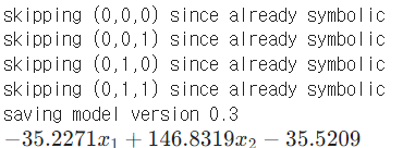
ex_round(formula2, 4)>>

# how accurate is this formula?
def acc(formula1, formula2, X, y):
    batch = X.shape[0]
    correct = 0
    for i in range(batch):
        logit1 = np.array(formula1.subs('x_1', X[i,0]).subs('x_2', X[i,1])).astype(np.float64)
        logit2 = np.array(formula2.subs('x_1', X[i,0]).subs('x_2', X[i,1])).astype(np.float64)
        correct += (logit2 > logit1) == y[i]
    return correct/batch

print('train acc of the formula:', acc(formula1, formula2, dataset['train_input'], dataset['train_label']))
print('test acc of the formula:', acc(formula1, formula2, dataset['test_input'], dataset['test_label']))
>>
train acc of the formula: tensor(0.8770)
test acc of the formula: tensor(0.8720)
Example 5 : Special functions
special function : $f(x, y) = exp(J_0(20x) + y^2)$, where $J_0(x)$ is the Bessel function
from kan import *

device = torch.device('cuda' if torch.cuda.is_available() else 'cpu')
print(device)

# create a KAN: 2D inputs, 1D output, and 5 hidden neurons. cubic spline (k=3), 5 grid intervals (grid=5).
model = KAN(width=[2,1,1], grid=3, k=3, seed=2, device=device)
f = lambda x: torch.exp(torch.special.bessel_j0(20*x[:,[0]]) + x[:,[1]]**2)
dataset = create_dataset(f, n_var=2, device=device)

# train the model
model.fit(dataset, opt="LBFGS", steps=20);
model.plot()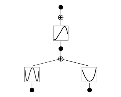
왼쪽 아래가 베셀 함수 model = model.refine(20) model.fit(dataset, opt="LBFGS", steps=20); model.plot()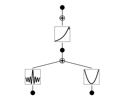
suggest_symbolic 함수가 기본 SYMBOLIC_LIB에 베셀 함수가 포함되어 있지 않기 때문에 일치하는 결과를 반환하지 않는다. 따라서 베셀 함수를 SYMBOLIC_LIB에 추가하려고 한다.
model.suggest_symbolic(0,0,0)
>>
  function  fitting r2   r2 loss  complexity  complexity loss  total loss
0        0    0.000000  0.000014           0                0    0.000003
1        x    0.001589 -0.002279           1                1    0.799544
2      cos    0.161514 -0.254125           2                2    1.549175
3      sin    0.161514 -0.254125           2                2    1.549175
4    1/x^2    0.099373 -0.150982           2                2    1.569804
('0',
 (<function kan.utils.<lambda>(x)>,
  <function kan.utils.<lambda>(x)>,
  0,
  <function kan.utils.<lambda>(x, y_th)>),
 0.0,
 0)
SYMBOLIC_LIB.keys() >> dict_keys(['x', 'x^2', 'x^3', 'x^4', 'x^5', '1/x', '1/x^2', '1/x^3', '1/x^4', '1/x^5', 'sqrt', 'x^0.5', 'x^1.5', '1/sqrt(x)', '1/x^0.5', 'exp', 'log', 'abs', 'sin', 'cos', 'tan', 'tanh', 'sgn', 'arcsin', 'arccos', 'arctan', 'arctanh', '0', 'gaussian'])베젤 함수를 SYMBOLIC_LIB에 추가하려면, 해당 함수의 이름, PyTorch 구현, 그리고 복잡도(c값)를 함께 정의해야 한다.
add_symbolic('J0', torch.special.bessel_j0, c=1)# J0 fitting is not very good model.suggest_symbolic(0,0,0) >> function fitting r2 r2 loss complexity complexity loss total loss 0 0 0.000000 0.000014 0 0 0.000003 1 J0 0.198534 -0.319268 1 1 0.736146 2 x 0.001589 -0.002279 1 1 0.799544 3 cos 0.161514 -0.254125 2 2 1.549175 4 sin 0.161514 -0.254125 2 2 1.549175 ('0', (<function kan.utils.<lambda>(x)>, <function kan.utils.<lambda>(x)>, 0, <function kan.utils.<lambda>(x, y_th)>), 0.0, 0)적합된 $R^2$ 값이 여전히 높지 않은 이유는, 실제 함수가 $J_0(20x)$인데 여기서 20이라는 값이 너무 크기 때문이다. 기본 검색 범위가(-10, 10)이므로 20을 포함하기 위해 검색 범위를 더 크게 설정해야 한다. 이제 $J_0$가 목록의 상단에 나타난다.
model.suggest_symbolic(0,0,0,a_range=(-40,40))
>>
  function  fitting r2   r2 loss  complexity  complexity loss  total loss
0       J0    0.998935 -9.862066           1                1   -1.172413
1        0    0.000000  0.000014           0                0    0.000003
2        x    0.001589 -0.002279           1                1    0.799544
3      cos    0.584193 -1.265980           2                2    1.346804
4      sin    0.584193 -1.265980           2                2    1.346804
('J0',
 (<function torch._C._special.special_bessel_j0>,
  J0,
  1,
  <function torch._C._special.special_bessel_j0>),
 0.9989354610443115,
 1)
Example 7 : Solving Partial Differential Equation(PDE) - tutorial과 같은 결과 X
$ \nabla^2 f(x, y) = -2\pi^2 \sin(\pi x) \sin(\pi y)$ with the boundary conditions $ f(-1, y) = f(1, y) = f(x, -1) = f(x, 1) = 0$. The ground truth solution is $ f(x, y) = \sin(\pi x) \sin(\pi y) $
from kan import * import matplotlib.pyplot as plt from torch import autograd from tqdm import tqdm device = torch.device('cuda' if torch.cuda.is_available() else 'cpu') print(device) dim = 2 np_i = 21 # number of interior points (along each dimension) np_b = 21 # number of boundary points (along each dimension) ranges = [-1, 1] model = KAN(width=[2,2,1], grid=5, k=3, seed=1, device=device) def batch_jacobian(func, x, create_graph=False): # x in shape (Batch, Length) def _func_sum(x): return func(x).sum(dim=0) return autograd.functional.jacobian(_func_sum, x, create_graph=create_graph).permute(1,0,2) # define solution sol_fun = lambda x: torch.sin(torch.pi*x[:,[0]])*torch.sin(torch.pi*x[:,[1]]) source_fun = lambda x: -2*torch.pi**2 * torch.sin(torch.pi*x[:,[0]])*torch.sin(torch.pi*x[:,[1]]) # interior sampling_mode = 'random' # 'radnom' or 'mesh' x_mesh = torch.linspace(ranges[0],ranges[1],steps=np_i) y_mesh = torch.linspace(ranges[0],ranges[1],steps=np_i) X, Y = torch.meshgrid(x_mesh, y_mesh, indexing="ij") if sampling_mode == 'mesh': #mesh x_i = torch.stack([X.reshape(-1,), Y.reshape(-1,)]).permute(1,0) else: #random x_i = torch.rand((np_i**2,2))*2-1 x_i = x_i.to(device) # boundary, 4 sides helper = lambda X, Y: torch.stack([X.reshape(-1,), Y.reshape(-1,)]).permute(1,0) xb1 = helper(X[0], Y[0]) xb2 = helper(X[-1], Y[0]) xb3 = helper(X[:,0], Y[:,0]) xb4 = helper(X[:,0], Y[:,-1]) x_b = torch.cat([xb1, xb2, xb3, xb4], dim=0) x_b = x_b.to(device) steps = 20 alpha = 0.01 log = 1 def train(): optimizer = LBFGS(model.parameters(), lr=1, history_size=10, line_search_fn="strong_wolfe", tolerance_grad=1e-32, tolerance_change=1e-32, tolerance_ys=1e-32) pbar = tqdm(range(steps), desc='description', ncols=100) for _ in pbar: def closure(): global pde_loss, bc_loss optimizer.zero_grad() # interior loss sol = sol_fun(x_i) sol_D1_fun = lambda x: batch_jacobian(model, x, create_graph=True)[:,0,:] sol_D1 = sol_D1_fun(x_i) sol_D2 = batch_jacobian(sol_D1_fun, x_i, create_graph=True)[:,:,:] lap = torch.sum(torch.diagonal(sol_D2, dim1=1, dim2=2), dim=1, keepdim=True) source = source_fun(x_i) pde_loss = torch.mean((lap - source)**2) # boundary loss bc_true = sol_fun(x_b) bc_pred = model(x_b) bc_loss = torch.mean((bc_pred-bc_true)**2) loss = alpha * pde_loss + bc_loss loss.backward() return loss if _ % 5 == 0 and _ < 50: model.update_grid_from_samples(x_i) optimizer.step(closure) sol = sol_fun(x_i) loss = alpha * pde_loss + bc_loss l2 = torch.mean((model(x_i) - sol)**2) if _ % log == 0: pbar.set_description("pde loss: %.2e | bc loss: %.2e | l2: %.2e " % (pde_loss.cpu().detach().numpy(), bc_loss.cpu().detach().numpy(), l2.cpu().detach().numpy())) train()더보기1. tqdm : Python에서 사용하는 진행률 표시바 라이브러리
2. torch.meshgrid에서 indexing = "ij"란? meshgrid를 만들 때 행렬 인덱싱 방식을 사용하겠다는 의미로 indexing옵션에는 두 가지가 있다.
(1) "ij" : 수학에서의 인덱스 표기법으로 첫 번째 좌표가 행(row), 두 번째 좌표가 열(column/)
(2) "xy" : 좌표 평면 인덱싱 방식으로 첫 번째 좌표가 x-좌표, 두 번째 좌표가 y-좌표
3. batch_jacobian 함수 : 주어진 함수의 입력에 대한 배치 자코비안 계산
def batch_jacobian(func, x, create_graph=False):
    # x in shape (Batch, Length)
    def _func_sum(x):
        return func(x).sum(dim=0)
    return autograd.functional.jacobian(_func_sum, x, create_graph=create_graph).permute(1,0,2)
x : [Batch, Length]
create_graph : 미분된 결과를 바탕으로 다시 미분이 가능하도록 그래프를 생성할지 여부를 결정하는 플래그. True로 설정하면 2차 미분 계산이 가능하다.
permute(1, 0, 2) : [Batch, Output, Input] 형식으로 맞춤
import torch
from torch import autograd

# batch_jacobian 함수 정의
def batch_jacobian(func, x, create_graph=False):
    def _func_sum(x):
        return func(x).sum(dim=0)
    return autograd.functional.jacobian(_func_sum, x, create_graph=create_graph).permute(1,0,2)

# 함수 정의: 입력 x의 각 요소를 제곱하여 반환
def example_func(x):
    # x의 각 요소를 제곱하여 반환
    return x ** 2

# 배치 데이터 생성: 3개의 샘플, 각 샘플은 2차원 벡터
x = torch.tensor([[1.0, 2.0], [3.0, 4.0], [5.0, 6.0]], requires_grad=True)

# batch_jacobian을 사용하여 example_func의 자코비안 계산
jacobian = batch_jacobian(example_func, x)

print("Input x:")
print(x)
print("\nJacobian:")
print(jacobian)
>>
Input x:
tensor([[1., 2.],
        [3., 4.],
        [5., 6.]], requires_grad=True)

Jacobian:
tensor([[[ 2.,  0.],
         [ 0.,  4.]],

        [[ 6.,  0.],
         [ 0.,  8.]],

        [[10.,  0.],
         [ 0., 12.]]])
4. pbar란? tqdm을 통해 생성된 진행률 표시
model.plot(beta=10)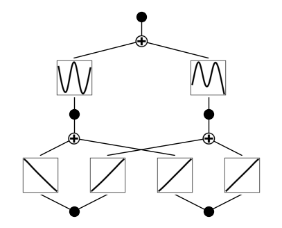
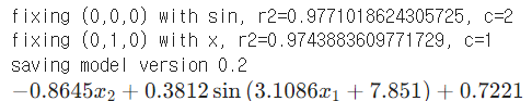
첫 번째 레이어의 활성화 함수는 선형 함수로, 두 번째 레이어의 활성화 함수는 사인 함수로 고정하자.(※하이퍼파라미터에 매우 민감할 수 있음)
model.fix_symbolic(0,0,0,'x')
model.fix_symbolic(0,0,1,'x')
model.fix_symbolic(0,1,0,'x')
model.fix_symbolic(0,1,1,'x')
>>
r2 is 0.9995107650756836
saving model version 0.1
r2 is 0.9994319677352905
saving model version 0.2
r2 is 0.999911367893219
saving model version 0.3
Best value at boundary.
r2 is 0.9999406933784485
saving model version 0.4
tensor(0.9999)
모든 레이어를 심볼릭 함수로 설정한 후, 모델을 추가로 훈련시키자.
train()
formula = model.symbolic_formula()[0][0]
ex_round(formula,6)
from kan import KAN, LBFGS import torch import matplotlib.pyplot as plt from torch import autograd from tqdm import tqdm device = torch.device('cuda' if torch.cuda.is_available() else 'cpu') print(device) dim = 2 np_i = 51 # number of interior points (along each dimension) np_b = 51 # number of boundary points (along each dimension) ranges = [-1, 1] def batch_jacobian(func, x, create_graph=False): # x in shape (Batch, Length) def _func_sum(x): return func(x).sum(dim=0) return autograd.functional.jacobian(_func_sum, x, create_graph=create_graph).permute(1,0,2) # define solution sol_fun = lambda x: torch.sin(torch.pi*x[:,[0]])*torch.sin(torch.pi*x[:,[1]]) source_fun = lambda x: -2*torch.pi**2 * torch.sin(torch.pi*x[:,[0]])*torch.sin(torch.pi*x[:,[1]]) # interior sampling_mode = 'mesh' # 'radnom' or 'mesh' x_mesh = torch.linspace(ranges[0],ranges[1],steps=np_i) y_mesh = torch.linspace(ranges[0],ranges[1],steps=np_i) X, Y = torch.meshgrid(x_mesh, y_mesh, indexing="ij") if sampling_mode == 'mesh': #mesh x_i = torch.stack([X.reshape(-1,), Y.reshape(-1,)]).permute(1,0) else: #random x_i = torch.rand((np_i**2,2))*2-1 x_i = x_i.to(device) # boundary, 4 sides helper = lambda X, Y: torch.stack([X.reshape(-1,), Y.reshape(-1,)]).permute(1,0) xb1 = helper(X[0], Y[0]) xb2 = helper(X[-1], Y[0]) xb3 = helper(X[:,0], Y[:,0]) xb4 = helper(X[:,0], Y[:,-1]) x_b = torch.cat([xb1, xb2, xb3, xb4], dim=0) x_b = x_b.to(device) alpha = 0.01 log = 1 grids = [5,10,20] steps = 50 pde_losses = [] bc_losses = [] l2_losses = [] for grid in grids: if grid == grids[0]: model = KAN(width=[2,2,1], grid=grid, k=3, seed=1, device=device) model = model.speed() else: model.save_act = True model.get_act(x_i) model = model.refine(grid) model = model.speed() def train(): optimizer = LBFGS(model.parameters(), lr=1, history_size=10, line_search_fn="strong_wolfe", tolerance_grad=1e-32, tolerance_change=1e-32, tolerance_ys=1e-32) pbar = tqdm(range(steps), desc='description', ncols=100) for _ in pbar: def closure(): global pde_loss, bc_loss optimizer.zero_grad() # interior loss sol = sol_fun(x_i) sol_D1_fun = lambda x: batch_jacobian(model, x, create_graph=True)[:,0,:] sol_D1 = sol_D1_fun(x_i) sol_D2 = batch_jacobian(sol_D1_fun, x_i, create_graph=True)[:,:,:] lap = torch.sum(torch.diagonal(sol_D2, dim1=1, dim2=2), dim=1, keepdim=True) source = source_fun(x_i) pde_loss = torch.mean((lap - source)**2) # boundary loss bc_true = sol_fun(x_b) bc_pred = model(x_b) bc_loss = torch.mean((bc_pred-bc_true)**2) loss = alpha * pde_loss + bc_loss loss.backward() return loss if _ % 5 == 0 and _ < 20: model.update_grid_from_samples(x_i) optimizer.step(closure) sol = sol_fun(x_i) loss = alpha * pde_loss + bc_loss l2 = torch.mean((model(x_i) - sol)**2) if _ % log == 0: pbar.set_description("pde loss: %.2e | bc loss: %.2e | l2: %.2e " % (pde_loss.cpu().detach().numpy(), bc_loss.cpu().detach().numpy(), l2.cpu().detach().numpy())) pde_losses.append(pde_loss.cpu().detach().numpy()) bc_losses.append(bc_loss.cpu().detach().numpy()) l2_losses.append(l2.cpu().detach().numpy()) train()plt.plot(pde_losses, marker='o') plt.plot(bc_losses, marker='o') plt.plot(l2_losses, marker='o') plt.yscale('log') plt.xlabel('steps') plt.legend(['PDE loss', 'BC loss', 'L2 squared'])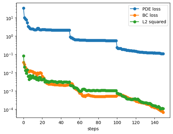
Example 8 : Continual Learning
우리의 목표는 샘플을 통해 1차원 함수를 학습하는 것이다. 이 1차원 함수는 5개의 가우시간 피크를 가지고 있다. 모든 샘플은 한 번에 신경망에 제공되는 대신, 다섯 단계에 걸쳐 학습을 진행한다. 각 단계에서는 하나의 피크 주변의 샘플만 KAN에 제공된다. 우리는 스플라인의 국소성 덕분에 KAN이 연속 학습을 수행할 수 있음을 발견했다.